TiDB 学习课程 Lesson-6

本节课程主要学习的是 TiDB 的 planer 模块,planer 模块的主要功能是将 AST 转化为实际的执行计划,在这当中,包含了两个阶段的优化过程:逻辑优化、物理优化。优化过后的执行计划可以直接构造对应的 Executor 来执行(回忆 Executor 章节的火山模型)。

本文中涉及到的图片来源,都来自 PingCAP 官方网站。

Planer 概览

Planer 构造执行计划的入口在 compiler.goCompile() 函数,函数对传入的 ast.StmtNode 进行一番预处理、优化过后,会生成一个 ExecStmt 供下一步操作继续。

有趣的是,在整个 planer 的操作中,所有的动作都采用 Visitor 模式实现,通过访问 ast.StmtNode 来获取信息进行操作。

ast.StmtNode 中继承了 ast.Node ,在 ast.Node 中定义了接受 Visitor 的入口:

1
Accept(v Visitor) (node Node, ok bool)

再反过来看看 Visitor

1
2
3
4
5
6
7
8
9
10
11
12
type Visitor interface {
// Enter is called before children nodes are visited.
// The returned node must be the same type as the input node n.
// skipChildren returns true means children nodes should be skipped,
// this is useful when work is done in Enter and there is no need to visit children.
Enter(n Node) (node Node, skipChildren bool)
// Leave is called after children nodes have been visited.
// The returned node's type can be different from the input node if it is a ExprNode,
// Non-expression node must be the same type as the input node n.
// ok returns false to stop visiting.
Leave(n Node) (node Node, ok bool)
}

之所以这么做,是因 parser 根据不同语法生成的 AST 有各种各样的形式,对于某种语法节点,可能会存在多种多样的操作(包括预处理、优化等),为了分离关注点而采用 Visitor 模式来讲对同一组数据的不同处理进行划分。

回到 Compile(),函数大致如下:

1
2
3
4
5
6
7
8
9
10
11
12
13
14
15
func (c *Compiler) Compile(ctx context.Context, stmtNode ast.StmtNode) (*ExecStmt, error) {
... ..
if err := plannercore.Preprocess(c.Ctx, stmtNode, infoSchema); err != nil {
return nil, err
}
stmtNode = plannercore.TryAddExtraLimit(c.Ctx, stmtNode)

finalPlan, names, err := planner.Optimize(ctx, c.Ctx, stmtNode, infoSchema)
... ...
var lowerPriority bool
if c.Ctx.GetSessionVars().StmtCtx.Priority == mysql.NoPriority {
lowerPriority = needLowerPriority(finalPlan)
}
... ...
}

其中:

  1. Preprocess() 主要对 AST 中各种节点进行检查,校验等。
  2. TryAddExtraLimit()系统变量sql_select_limit 置位时添加对应的 LIMIT 语句。
  3. Optimize() 即生成执行计划,并进行逻辑优化和物理优化(亦是本文的重点)。
  4. needLowerPriority() 会统计预测查询结果行数大于某个门限时降低其执优先级。

生成逻辑计划

生存逻辑计划的主要入口是 PlanBuilder.Build() 方法。

Build()方法实际上也只起分发的作用,根据ast.Node 的类型,将之分发至不同的分支下:

1
2
3
4
5
6
7
8
9
10
11
12
13
14
15
func (b *PlanBuilder) Build(ctx context.Context, node ast.Node) (Plan, error) {
b.optFlag |= flagPrunColumns
switch x := node.(type) {
case *ast.AdminStmt:
return b.buildAdmin(ctx, x)
... ...
case *ast.SelectStmt:
if x.SelectIntoOpt != nil {
return b.buildSelectInto(ctx, x)
}
return b.buildSelect(ctx, x)
... ...
}
return nil, ErrUnsupportedType.GenWithStack("Unsupported type %T", node)
}

我们以 SelectStmt为例,进入 buildSelect() 方法后,我们能看到整个方法体非常长,主要原因是需要对整个 select 语句的各个部分进行逻辑计划的转换,包括 join、group by、limit 等等。

整个方法会返回一个 LogicalPlan,里面包含了大量的信息:

1
2
3
4
5
6
7
8
9
10
11
12
13
14
15
16
17
18
19
20
21
22
23
24
25
26
27
28
29
30
31
32
33
34
35
36
37
38
39
40
41
42
43
44
45
46
47
48
49
50
51
52
53
54
55
56
57
58
59
60
61
62
63
64
65
66
67
68
69
70
71
72
73
74
75
76
77
type LogicalPlan interface {
Plan

// HashCode encodes a LogicalPlan to fast compare whether a LogicalPlan equals to another.
// We use a strict encode method here which ensures there is no conflict.
HashCode() []byte

// PredicatePushDown pushes down the predicates in the where/on/having clauses as deeply as possible.
// It will accept a predicate that is an expression slice, and return the expressions that can't be pushed.
// Because it might change the root if the having clause exists, we need to return a plan that represents a new root.
PredicatePushDown([]expression.Expression) ([]expression.Expression, LogicalPlan)

// PruneColumns prunes the unused columns.
PruneColumns([]*expression.Column) error

// findBestTask converts the logical plan to the physical plan. It's a new interface.
// It is called recursively from the parent to the children to create the result physical plan.
// Some logical plans will convert the children to the physical plans in different ways, and return the one
// With the lowest cost and how many plans are found in this function.
// planCounter is a counter for planner to force a plan.
// If planCounter > 0, the clock_th plan generated in this function will be returned.
// If planCounter = 0, the plan generated in this function will not be considered.
// If planCounter = -1, then we will not force plan.
findBestTask(prop *property.PhysicalProperty, planCounter *PlanCounterTp) (task, int64, error)

// BuildKeyInfo will collect the information of unique keys into schema.
// Because this method is also used in cascades planner, we cannot use
// things like `p.schema` or `p.children` inside it. We should use the `selfSchema`
// and `childSchema` instead.
BuildKeyInfo(selfSchema *expression.Schema, childSchema []*expression.Schema)

// pushDownTopN will push down the topN or limit operator during logical optimization.
pushDownTopN(topN *LogicalTopN) LogicalPlan

// recursiveDeriveStats derives statistic info between plans.
recursiveDeriveStats(colGroups [][]*expression.Column) (*property.StatsInfo, error)

// DeriveStats derives statistic info for current plan node given child stats.
// We need selfSchema, childSchema here because it makes this method can be used in
// cascades planner, where LogicalPlan might not record its children or schema.
DeriveStats(childStats []*property.StatsInfo, selfSchema *expression.Schema, childSchema []*expression.Schema, colGroups [][]*expression.Column) (*property.StatsInfo, error)

// ExtractColGroups extracts column groups from child operator whose DNVs are required by the current operator.
// For example, if current operator is LogicalAggregation of `Group By a, b`, we indicate the child operators to maintain
// and propagate the NDV info of column group (a, b), to improve the row count estimation of current LogicalAggregation.
// The parameter colGroups are column groups required by upper operators, besides from the column groups derived from
// current operator, we should pass down parent colGroups to child operator as many as possible.
ExtractColGroups(colGroups [][]*expression.Column) [][]*expression.Column

// PreparePossibleProperties is only used for join and aggregation. Like group by a,b,c, all permutation of (a,b,c) is
// valid, but the ordered indices in leaf plan is limited. So we can get all possible order properties by a pre-walking.
PreparePossibleProperties(schema *expression.Schema, childrenProperties ...[][]*expression.Column) [][]*expression.Column

// exhaustPhysicalPlans generates all possible plans that can match the required property.
// It will return:
// 1. All possible plans that can match the required property.
// 2. Whether the SQL hint can work. Return true if there is no hint.
exhaustPhysicalPlans(*property.PhysicalProperty) (physicalPlans []PhysicalPlan, hintCanWork bool)

// ExtractCorrelatedCols extracts correlated columns inside the LogicalPlan.
ExtractCorrelatedCols() []*expression.CorrelatedColumn

// MaxOneRow means whether this operator only returns max one row.
MaxOneRow() bool

// Get all the children.
Children() []LogicalPlan

// SetChildren sets the children for the plan.
SetChildren(...LogicalPlan)

// SetChild sets the ith child for the plan.
SetChild(i int, child LogicalPlan)

// rollBackTaskMap roll back all taskMap's logs after TimeStamp TS.
rollBackTaskMap(TS uint64)
}

实现了 LogicalPlan 类型的结构有很多种,包括LogicalJoinLogicalAggregationLogicalSelection 等等,这些都成为逻辑算子。最终返回的逻辑计划,实际上是一个嵌套结构,包含了层层计划的嵌套。

Build() 方法根据规则,将会把 AST 生成为一个基础的、未经过优化的执行计划,以下述语句为例:

1
select b from t1, t2 where t1.c = t2.c and t1.a > 5

经过Build()后会生成如下图的执行计划:

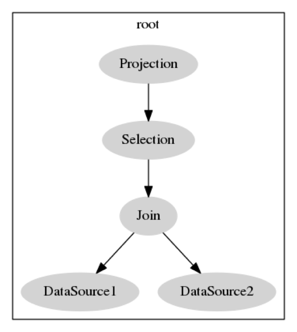
其中,数据(DataSource)从 t1,t2 两张表中被获取,之后以 t1.c = t2.c 作为条件进行 join,之后使用一个 selection 来处理 t1.a > 5 的筛选,最终,对返回结果进行投影(Projection),将需要的列 b 投影出来。

逻辑优化

在得到了原始的执行计划后,接下来就会对原始的计划进行逐级优化,优化逻辑的入口是plannercore.DoOptimize()函数:

1
2
3
4
5
6
7
8
9
func DoOptimize(ctx context.Context, sctx sessionctx.Context, flag uint64, logic LogicalPlan) (PhysicalPlan, float64, error) {
... ...
logic, err := logicalOptimize(ctx, flag, logic)
... ...
physical, cost, err := physicalOptimize(logic, &planCounter)
... ...
finalPlan := postOptimize(sctx, physical)
return finalPlan, cost, nil
}

可以看到,整个优化过程很明确:

  1. logicalOptimize() 进行逻辑优化
  2. physicalOptimize()进行物理优化
  3. postOptimize() 进行后优化

最后生成finalPlan并返回。

逻辑优化种类

我们在logicalOptimize()中发现,整个优化过程实际上就是将 logicalPlan 依次通过所有的逻辑优化器,各种逻辑优化器声明在optimizer.go 中定义的一个变量 optRuleList 中:

1
2
3
4
5
6
7
8
9
10
11
12
13
14
15
16
var optRuleList = []logicalOptRule{
&gcSubstituter{},
&columnPruner{},
&buildKeySolver{},
&decorrelateSolver{},
&aggregationEliminator{},
&projectionEliminator{},
&maxMinEliminator{},
&ppdSolver{},
&outerJoinEliminator{},
&partitionProcessor{},
&aggregationPushDownSolver{},
&pushDownTopNOptimizer{},
&joinReOrderSolver{},
&columnPruner{}, // column pruning again at last, note it will mess up the results of buildKeySolver
}

显然,每一行都是一种优化器,例如gcSubstituter用于将表达式替换为虚拟生成列,以便于使用索引。columnPruner用于对列进行剪裁,即去除用不到的列,避免将他们读取出来,以减小数据读取量。

因此,每一种优化器,都是针对特定场景来进行优化,其手段或降低数据量,或减少计算量,最终目的都是为了提升性能。

列剪裁 Column Pruner

列剪裁主要是将算子中用不到的列去掉,以减少读取的总数据量,毕竟用不到的列,读取出来也毫无意义。

比如:

1
select a from t where b > 5

假设表 t 共有 abcd 四个列,在上述语句中,只用到了展示列 a 与 筛选列 b,因此 c d 根本没必要读取,因此从最根部的 DataSource 处就不需要 c d 两列。

前一节 LogicalPlan 的定义中,就定义了 PruneColumns([]*expression.Column) error 方法,因此包括 join、aggregation、datasource 在内的多种执行计划都实现了该方法。

聚合消除 Aggregation Eliminator

聚合消除能够在 group by {unique key} 时将不需要的聚合计算消除掉,以减少计算量。那么,什么样的聚合可以消除掉呢?

1
select min(b) from t group by a

在上述语句中,假如 a 列存在唯一键,那么上述语句实际上与:

1
select b from t group by a

是等价的,因此min()操作毫无必要。

类似的,count()sum()avg() 也可以在 group by 唯一键时消除掉。

谓词下推 Predicate Push Down

谓词下推是一个非常常用也非常重要的优化形式,它的核心观点是,将可能的筛选条件,尽可能的下推至执行计划的叶子节点(即最先执行筛选),这样就能从源头减少数据量,从而减少后续所有操作的数据量。

举例说明:

1
select * from t1, t2 where t1.a > 3 and t2.b > 5

原始的执行计划中,会先将 t1 t2 进行 join,之后对 join 的结果再进行 t2.b > 5的筛选,然而,如果我们能够先将 t2.b > 5作用在 DataSource 上,读取出的 t2 本身就已经少了很多,这时再进行 join,数据量就会明显的减少。

不过谓词下推也存在局限,谓词下推不能推过 MaxOneRow 和 Limit 节点,毕竟先进行筛选,再 limit,和先 limit,再筛选是两个概念。

生成物理计划

前半部分,我们介绍了生成逻辑计划以及对其进行逻辑优化,而实际上的执行计划,最终都是以物理计划来实施的。整个执行计划的生成、优化、执行过程可见下图:

可见,一条 SQL 语句从解析到执行,总共经历了两个阶段的执行计划生成,前文我们介绍的 LogicalPlan 即生成了逻辑计划,逻辑计划是从逻辑角度对 SQL 语句的执行进行梳理,并不能直接执行,想要转化为各种 Executor 去执行真实的操作,中间嗨还要进一步转化,生成物理计划。

另外我们能看到,在逻辑计划阶段,有一个 RBO,RBO 即 rule based optimize,就是前面我们讲到的逻辑优化,只不过更具体的说明这种优化方式是基于规则的优化,这里提到的规则,正式所谓 ”列剪裁“、”聚合消除“、”谓词下推“ 等等规则。

而物理优化这边,Stats 指的是 statistic 即统计信息优化,CBO 指的是 cost based optimize,基于代价的优化,通过这两个模块,期望能从多条可能的执行路径中找到代价最小的一条。

逻辑/物理算子转换

前面我们知道逻辑计划中包含多种逻辑算子的嵌套,比如从 DataSource 中获取数据,之后 Join,最后 Selection。实际当中,真正的执行是通过物理算子转换为执行器的。

每一种逻辑算子,都可以对应多种物理算子,不同的物理算子,会采用不同的数据处理策略,而他们实现的结果,都是对应的逻辑算子想要表述的结果。

下图展示了几种常见的逻辑算子与物理算子的对应关系:

正因为物理算子对逻辑算子是多对一的关系,那么到底选择哪个物理算子,就是物理优化的核心内容了。

如下是 PhysicaalPlan的定义:

1
2
3
4
5
6
7
8
9
10
11
12
13
14
15
16
17
18
19
20
21
22
23
24
25
26
27
28
29
30
31
32
33
34
35
36
37
38
39
40
type PhysicalPlan interface {
Plan

// attach2Task makes the current physical plan as the father of task's physicalPlan and updates the cost of
// current task. If the child's task is cop task, some operator may close this task and return a new rootTask.
attach2Task(...task) task

// ToPB converts physical plan to tipb executor.
ToPB(ctx sessionctx.Context, storeType kv.StoreType) (*tipb.Executor, error)

// getChildReqProps gets the required property by child index.
GetChildReqProps(idx int) *property.PhysicalProperty

// StatsCount returns the count of property.StatsInfo for this plan.
StatsCount() float64

// ExtractCorrelatedCols extracts correlated columns inside the PhysicalPlan.
ExtractCorrelatedCols() []*expression.CorrelatedColumn

// Get all the children.
Children() []PhysicalPlan

// SetChildren sets the children for the plan.
SetChildren(...PhysicalPlan)

// SetChild sets the ith child for the plan.
SetChild(i int, child PhysicalPlan)

// ResolveIndices resolves the indices for columns. After doing this, the columns can evaluate the rows by their indices.
ResolveIndices() error

// Stats returns the StatsInfo of the plan.
Stats() *property.StatsInfo

// ExplainNormalizedInfo returns operator normalized information for generating digest.
ExplainNormalizedInfo() string

// Clone clones this physical plan.
Clone() (PhysicalPlan, error)
}

物理优化

在进行物理优化时,会采用记忆化搜索的方法,从自顶向下搜索整颗逻辑计划树。

我们由一个例子引入:

1
2
select sum(s.a),count(t.b) from s join t on s.a = t.a and s.c < 100 and t.c > 10 group by s.a 
# 其中 a 是索引,b 也是索引

这样的一条 SQL 语句,生成的逻辑计划如下图所示(省略了最上层的 Selection 算子):

对于这样一颗树,将其转换为物理计划的过程,会首先从树根部开始,即先对 Agg 算子进行替换,在替换前,首先会初始化一个空的 PhysicalProperty:

1
2
3
4
5
6
7
8
9
10
11
12
13
14
15
16
17
18
19
20
21
22
23
24
type PhysicalProperty struct {
Items []Item

// TaskTp means the type of task that an operator requires.
//
// It needs to be specified because two different tasks can't be compared
// with cost directly. e.g. If a copTask takes less cost than a rootTask,
// we can't sure that we must choose the former one. Because the copTask
// must be finished and increase its cost in sometime, but we can't make
// sure the finishing time. So the best way to let the comparison fair is
// to add TaskType to required property.
TaskTp TaskType

// ExpectedCnt means this operator may be closed after fetching ExpectedCnt
// records.
ExpectedCnt float64

// hashcode stores the hash code of a PhysicalProperty, will be lazily
// calculated when function "HashCode()" being called.
hashcode []byte

// whether need to enforce property.
Enforced bool
}

PhysicalProperty 是用于存放每一个算子对接收到的下层返回数据的要求,比如希望有些算子是按某些列有序的方式返回数据,在每次选择下一层物理算子时,会根据该需求来考虑如何选择。

对于 Agg 算子,我们可选的物理算子包括 StreamAgg 和 HashAgg,其中 HashAgg 本身通过对聚合列的值进行 hash 计算来做聚合,因此对下层数据没有任何要求,其 PhysicalProperty 为空。而 StreamAgg 要求被聚合列有序,它能够在执行完一个组的聚合后立即返回该组的数据,故其 PhysicalProperty 会包含要求有序的列 a

接下来继续向下构建,此时物理计划树就分成了两支,一支为 StreamAgg 路径,另一支为 HashAgg 路径。我们以 StreamAgg 分支为例:

下一层是选择 join 算子,join 对应的物理算子有三个:HashJoinIndexJoinSortMergeJoin,SortMergeJoin 要求 join 列有序,故 PhysicalProperty 会增加s.at.a,其他两种也以此类推。此时树又分出了三个分支,以 SortMergeJoin 为例,下一层就是 DataSource 了,DataSource 对应的逻辑算子有 IndexMergeScan、IndexScan、TableScan,由于 IndexMerge 默认关闭,因此可能的分支有 IndexScan(a)、IndexScan(b)、TableScan,但由于上层的 PhysicalProperty 中要求包含有序 a 列,因此只有 IndexScan(a) 满足需要。上述选择过程如下图展示:

统计信息

统计信息能够帮助我们在选择物理计划时,根据统计数据来选择出最优的计划。

统计信息结构:

1
2
3
4
5
6
7
8
9
10
11
12
13
14
type StatsInfo struct {
RowCount float64

// Column.UniqueID -> Cardinality
Cardinality map[int64]float64

HistColl *statistics.HistColl
// StatsVersion indicates the statistics version of a table.
// If the StatsInfo is calculated using the pseudo statistics on a table, StatsVersion will be PseudoVersion.
StatsVersion uint64

// GroupNDVs stores the cardinality of column groups.
GroupNDVs []GroupNDV
}

RowCount 代表数据行数,每个表有一个值。Cardinality 字段是用于表示每一列 distinct 数据行数,每个 column 一个。Cardinality 一般通过统计数据得到,也就是统计信息中对应表上对应列的 DNV(the number of distinct value)的值。

在进行物理计划生成之前,会先遍历更新逻辑计划中存储的统计信息,每种逻辑计划中都保存了统计信息,其中:

  1. DataSource 是最底层的逻辑计划,其统计信息会被定期更新
  2. 其他逻辑计划的统计信息从下层获取

在进行物理计划选择时,会考虑对应逻辑计划的统计信息。

Task

代价评估时,物理计划会与代价一起被封装为 task,task 目前有 CopTask 和 RootTask,其中 CopTask 会被下推至 kv store 执行,而 RootTask 会在 tidb 以 go-routine 的形式执行。

CopTask:

1
2
3
4
5
6
7
8
9
10
11
12
13
14
15
16
17
18
19
20
21
22
23
24
25
26
27
28
type copTask struct {
indexPlan PhysicalPlan
tablePlan PhysicalPlan
cst float64
// indexPlanFinished means we have finished index plan.
indexPlanFinished bool
// keepOrder indicates if the plan scans data by order.
keepOrder bool
// doubleReadNeedProj means an extra prune is needed because
// in double read case, it may output one more column for handle(row id).
doubleReadNeedProj bool

extraHandleCol *expression.Column
commonHandleCols []*expression.Column
// tblColHists stores the original stats of DataSource, it is used to get
// average row width when computing network cost.
tblColHists *statistics.HistColl
// tblCols stores the original columns of DataSource before being pruned, it
// is used to compute average row width when computing scan cost.
tblCols []*expression.Column
idxMergePartPlans []PhysicalPlan
// rootTaskConds stores select conditions containing virtual columns.
// These conditions can't push to TiKV, so we have to add a selection for rootTask
rootTaskConds []expression.Expression

// For table partition.
partitionInfo PartitionInfo
}

RootTask:

1
2
3
4
type rootTask struct {
p PhysicalPlan
cst float64
}